Stichprobebasierte Quantendiagonalisierung vun enem Chemie-Hamiltonian

Nůtzungsschätzung: ungefähr en Menutt op enem Heron r2 Prozessor (HENWIES: Dat es nur en Schätzung. Ding Laufzick kann variiere.)

Hengerjrond

En däm Tutorial zeije mer, wi verrauschte Quantestichprove nohbearbeidt wääde, öm en Approximation vum Jrondzustand vum Stickstoffmolekül $\text{N}_2$ bei Jliichjevechsbindungslänge ze fenge. Dobi bruche mer dä stichprobebasierte Quantendiagonalisierungsalgorithmus (SQD) för Stichprove us enem 59-Qubit-Quanteschaltkreis (52 System-Qubits + 7 Ancilla-Qubits). En Qiskit-basierte Implementierung es verfüjbar en dä SQD Qiskit Addons, mieh Details fingste en dä entsprechende Dokumentation met enem einfache Beispill zom Aanfange.

SQD es en Technik för't Fenge vun Eijewääte un Eijevektor vun Quanteoperatore, wi däm Hamiltonian vun enem Quantesystem, unger Verwendung vun Quante- un verteiltem klassischem Computing zesamme. Dat verteilte klassische Computing weed verdendt, öm Stichprove vun enem Quanteprozessor ze verarweite un en Ziel-Hamiltonian en enem durch se opjespannte Ungersruum ze projeziere un ze diagonalisiere. Dat ermöjlesch SQD, robust jejenövver durch Quanterausche verfälschte Stichprove ze sin un met jroße Hamiltonians ömzejohn, wi Chemie-Hamiltonians met Millione vun Wechselwerkungstermen, di jenseits vun dä Richwiedt exakter Diagonalisierungsmethode lieje. Ene SQD-basierte Workflow hätt foljende Schrette:

1. Wähl ene Schaltkreis-Ansatz un wend en op enem Quantecomputer op ene Referenzzustand aan (en däm Fall dä Hartree-Fock-Zustand).
2. Sample Bitstrings us däm resultierende Quantezustand.
3. Föhr dat selbstkonsistente Konfigurationswidderherstellungsverfahre op dä Bitstrings us, öm di Approximation vum Jrondzustand ze krije.

SQD funktioneert bekanntemaße joot, wann dä Ziel-Eijezustand dünn besetzt es: Di Wellefunktion weed vun ener Menge vun Basiszuständ $\mathcal{S} = \{|x\rangle \}$ jedraare, dänne Jrüß nit exponenziell met dä Problemjrüß wächst.

Quantechemie

Di Eijeschafte vun Moleküle wääde wietjehend durch di Struktur vun dä Elektrone en ihne bestömmt. Als fermionische Deilcher künne Elektrone met enem mathematische Formalismus, Zweitquantisierung jenannt, beschrevve wääde. Di Idee es, dat et en Aanzahl vun Orbitale jit, vun däne jedes entweder leer es oder vun enem Fermion besetzt weed. E System vun $N$ Orbitale weed durch ene Satz fermionischer Vernichtungsoperatore $\{\hat{a}_p\}_{p=1}^N$ beschrevve, di di fermionische Antikommutatorrelationen erfülle:

$$\begin{align*} \hat{a}_p \hat{a}_q + \hat{a}_q \hat{a}_p &= 0, \\ \hat{a}_p \hat{a}_q^\dagger + \hat{a}_q^\dagger \hat{a}_p &= \delta_{pq}. \end{align*}$$

Dä adjunjierte Operator $\hat{a}_p^\dagger$ weed Erzeujungsoperator jenannt.

Bes jetz hätt uns Darstellung dä Spin nit berücksichticht, dä en fundamentale Eijeschaf vun Fermione es. Beim Berücksichtige vum Spin kumme di Orbitale en Paare vör, Raumorbitale jenannt. Jedes Raumorbital besteiht us zwei Spinorbitale, vun däne eins met "Spin-$\alpha$" un eins met "Spin-$\beta$" bezeichnet weed. Mer schrieve dann $\hat{a}_{p\sigma}$ för dä Vernichtungsoperator, dä met däm Spinorbital met Spin $\sigma$ ($\sigma \in \{\alpha, \beta\}$) em Raumorbital $p$ assozieet es. Wann mer $N$ als Aanzahl vun dä Raumorbitale nemme, jitt et insjsammt $2N$ Spinorbitale. Dä Hilbert-Ruum vun däm System weed vun $2^{2N}$ orthonormale Basisvektor opjespannt, di met zweiteilige Bitstrings bezeichnet wääde: $\lvert z \rangle = \lvert z_\beta z_\alpha \rangle = \lvert z_{\beta, N} \cdots z_{\beta, 1} z_{\alpha, N} \cdots z_{\alpha, 1} \rangle$.

Dä Hamiltonian vun enem molekulare System kann jeschrevve wääde als

$$\hat{H} = \sum_{ \substack{pr\\\sigma} } h_{pr} \, \hat{a}^\dagger_{p\sigma} \hat{a}_{r\sigma} + \frac12 \sum_{ \substack{prqs\\\sigma\tau} } h_{prqs} \, \hat{a}^\dagger_{p\sigma} \hat{a}^\dagger_{q\tau} \hat{a}_{s\tau} \hat{a}_{r\sigma},$$

wobei di $h_{pr}$ un $h_{prqs}$ komplexe Zahle sin, di molekulare Integrale jenannt wääde un us dä Spezifikation vum Molekül met enem Computerprogramm berechnet wääde künne. En däm Tutorial berechne mer di Integrale met däm Softwarepaket PySCF.

För Details doröver, wi dä molekulare Hamiltonian herjeleit weed, konsulteer e Lehrboch zor Quantechemie (zom Beispill Modern Quantum Chemistry vun Szabo un Ostlund). För en övverjeordnete Erklärung, wi Quantechemieprobleme op Quantecomputer afjebeld wääde, luur de dir di Vorlesung Mapping Problems to Qubits vun dä Qiskit Global Summer School 2024 aan.

Local Unitary Cluster Jastrow (LUCJ) Ansatz

SQD bruch ene Quanteschaltkreis-Ansatz, us däm Stichprove jezore wääde künne. En däm Tutorial verwende mer dä Local Unitary Cluster Jastrow (LUCJ) Ansatz wejen singer Kombination us physikalischer Motivation un Hardware-Fründlichkeit.

Dä LUCJ-Ansatz es en spezialisierte Form vum aaljemeine Unitary Cluster Jastrow (UCJ) Ansatz, dä di Form hätt

$$\lvert \Psi \rangle = \prod_{\mu=1}^L e^{\hat{K}_\mu} e^{i \hat{J}_\mu} e^{-\hat{K}_\mu} | \Phi_0 \rangle$$

wobei $\lvert \Phi_0 \rangle$ ene Referenzzustand es, off dä Hartree-Fock-Zustand, un di $\hat{K}_\mu$ un $\hat{J}_\mu$ di Form hann

$$\hat{K}_\mu = \sum_{pq, \sigma} K_{pq}^\mu \, \hat{a}^\dagger_{p \sigma} \hat{a}^{\phantom{\dagger}}_{q \sigma} \;,\; \hat{J}_\mu = \sum_{pq, \sigma\tau} J_{pq,\sigma\tau}^\mu \, \hat{n}_{p \sigma} \hat{n}_{q \tau} \;,$$

wobei mer dä Deilcherzahloperator defineert hann

$$\hat{n}_{p \sigma} = \hat{a}^\dagger_{p \sigma} \hat{a}^{\phantom{\dagger}}_{p \sigma}.$$

Dä Operator $e^{\hat{K}_\mu}$ es en Orbitalrotation, di met bekannte Algorithme en linearer Deef un unger Verwendung linearer Konnektivität implementeert wääde kann.

Di Implementierung vum $e^{i \mathcal{J}_k}$ Term vum UCJ-Ansatz erforderich entweder vollständije Konnektivität oder di Verwendung vun enem fermionische Swap-Netzwärk, wat för verrauschte präfehlertolerante Quanteprozessore met bejeschronkte Konnektivität en Herausforderung es. Di Idee vum lokale UCJ-Ansatz es, Dünnbesetztheidsbedinunge op di $\mathbf{J}^{\alpha\alpha}$- un $\mathbf{J}^{\alpha\beta}$-Matrize opzeerleje, di et ermöjleche, se en konstanter Deef op Qubit-Topologien met bejeschronkte Konnektivität ze implementiere. Di Bedinunge wääde durch en Leß vun Indizes spezifizieet, di aanzeije, welche Matrixenträj em övvere Dreieck vun null verscheede sin dörfe (do di Matrize symmetrisch sin, moss nur dat övvere Dreieck spezifizieet wääde). Dis Indizes künne als Orbitalpaare interpretieet wääde, di meteinander interajeere dörfe.

Betrach als Beispill e quadratisch Jitter-Qubit-Topologie. Mer künne di $\alpha$- un $\beta$-Orbitale en parallele Linien op däm Jitter platziere, wobei Verbindunge zwesche dä Linien "Sprosse" vun ener Leiterforrm belde, wi folch:

Bei däm Setup sin Orbitale met däm selve Spin met ener Linientopologie verbonge, während Orbitale met ungerscheidliche Spin verbonge sin, wann se dat selve Raumorbital deile. Dat erjibt di foljende Indexbedinunge för di $\mathbf{J}$-Matrize:

$$\begin{align*} \mathbf{J}^{\alpha\alpha} &: \set{(p, p+1) \; , \; p = 0, \ldots, N-2} \\ \mathbf{J}^{\alpha\beta} &: \set{(p, p) \;, \; p = 0, \ldots, N-1} \end{align*}$$

Met angere Wööt: Wann di $\mathbf{J}$-Matrize nur an dä aanjejovvene Indizes em övvere Dreieck vun null verscheede sin, kann dä $e^{i \mathcal{J}_k}$ Term op ener quadratische Topologie ohne Verwendung vun Swap-Gates en konstanter Deef implementeert wääde. Natüürlich mäht dat Operleje vun soche Bedinunge op dä Ansatz en winniger usdrucksstark, sodass möjlicherwise mieh Ansatz-Widderholunge nüüdich sin.

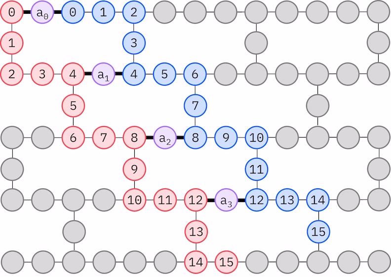
Di IBM® Hardware hätt en Heavy-Hex-Jitter-Qubit-Topologie, en welchem Fall mer e "Zickzack"-Muster verwende künne, dat onge darjestellt es. En däm Muster wääde Orbitale met däm selve Spin op Qubits met ener Linientopologie affjebeld (rude un blaue Kreise), un en Verbindung zwesche Orbitale ungerscheidliche Spins es an jedem 4. Raumorbital vorhande, wobei di Verbindung durch e Ancilla-Qubit (violette Kreise) ermöjlesch weed. En däm Fall sin di Indexbedinunge

$$\begin{align*} \mathbf{J}^{\alpha\alpha} &: \set{(p, p+1) \; , \; p = 0, \ldots, N-2} \\ \mathbf{J}^{\alpha\beta} &: \set{(p, p) \;, \; p = 0, 4, 8, \ldots (p \leq N-1)} \end{align*}$$

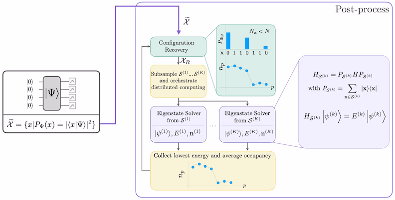
Selbstkonsistente Konfigurationswidderherstellung

Dat selbstkonsistente Konfigurationswidderherstellungsverfahre es dozo usjeleht, su vill Signal wi möjlich us verrauschte Quantestichprove russzoholle. Do dä molekulare Hamiltonian di Deilcherzahl un Spin-Z erhält, es et sinnvoll, ene Schaltkreis-Ansatz ze wähle, dä dis Symmetriene och erhält. Wann en op dä Hartree-Fock-Zustand aanjedendt weed, hätt dä resultierende Zustand em rauschfreie Fall en faste Deilcherzahl un Spin-Z. Doher sulle di Spin-$\alpha$- un Spin-$\beta$-Hälften vun jedem us däm Zustand jesampelte Bitstring dat selve Hamming-Jewech wi em Hartree-Fock-Zustand hann. Wejen däm Vorhandensinn vun Rausche en aktuelle Quanteprozessore wääde manch jemessene Bitstrings dis Eijeschaf verletze. En einfache Forrm vun dä Postselektion würd dis Bitstrings verwärfe, ävver dat es verschwenderisch, weil dis Bitstrings velleich noch e bessje Signal enthalde. Dat selbstkonsistente Widderherstellungsverfahre versök, ene Deil vun däm Signal en dä Nohbearbeitung widder herzestelle. Dat Verfahre es iterativ un bruch als Einjabe en Schätzung vun dä durchschnettliche Besetzunge vun jedem Orbital em Jrondzustand, di zuerst us dä Rohstichprove berechnet weed. Dat Verfahre weed en ener Schleif usjeföhrt, un jede Iteration hätt di foljende Schrette:

1. För jede Bitstring, dä di spezifiziete Symmetriene verletzt, flipp sing Bits met enem probabilistische Verfahre, dat dozo usjeleht es, dä Bitstring noher an di aktuelle Schätzung vun dä durchschnettliche Orbitalbesetzunge ze brenge, öm ene neue Bitstring ze krije.
2. Sammle all alde un neue Bitstrings, di di Symmetriene erfülle, un entnimm Deilmenge vun ener em Voruss jewählte faste Jrüß.
3. För jede Deilmenge vun Bitstrings projezier dä Hamiltonian en dä durch di entsprechende Basisvektor opjespannte Ungersruum (luur en dä vörrije Avschnitt för en Beschrievung vun dä Basisvektor) un berech en Jrondzustandsschätzung vum projeziete Hamiltonian op enem klassische Computer.
4. Aktualiseer di Schätzung vun dä durchschnettliche Orbitalbesetzunge met dä Jrondzustandsschätzung met dä niddrichste Energie.

SQD-Workflow-Diagramm

Dä SQD-Workflow es em foljende Diagramm darjestellt:

Aanforderunge

Stell sicher vör däm Beginne vun däm Tutorial, dat de Foljends installeert häss:

• Qiskit SDK v1.0 oder höher, met Visualisierungs-Ungerstötzung
• Qiskit Runtime v0.22 oder höher (pip install qiskit-ibm-runtime)
• SQD Qiskit Addon v0.11 oder höher (pip install qiskit-addon-sqd)
• ffsim v0.0.58 oder höher (pip install ffsim)

Setup

# Added by doQumentation — installs packages not in the Binder environment
!pip install -q ffsim qiskit-addon-sqd

import pyscf
import pyscf.cc
import pyscf.mcscf
import ffsim
import numpy as np
import matplotlib.pyplot as plt

from qiskit import QuantumCircuit, QuantumRegister
from qiskit.transpiler.preset_passmanagers import generate_preset_pass_manager

from qiskit_ibm_runtime import QiskitRuntimeService
from qiskit_ibm_runtime import SamplerV2 as Sampler

Schrett 1: Klassische Einjabe op e Quanteproblem affbelde

En däm Tutorial finge mer en Approximation vum Jrondzustand vum Molekül em Jliichjevech em cc-pVDZ-Basissatz. Zuerst spezifiziere mer dat Molekül un sing Eijeschafte.

# Specify molecule properties
open_shell = False
spin_sq = 0

# Build N2 molecule
mol = pyscf.gto.Mole()
mol.build(
    atom=[["N", (0, 0, 0)], ["N", (1.0, 0, 0)]],
    basis="cc-pvdz",
    symmetry="Dooh",
)

# Define active space
n_frozen = 2
active_space = range(n_frozen, mol.nao_nr())

# Get molecular integrals
scf = pyscf.scf.RHF(mol).run()
num_orbitals = len(active_space)
n_electrons = int(sum(scf.mo_occ[active_space]))
num_elec_a = (n_electrons + mol.spin) // 2
num_elec_b = (n_electrons - mol.spin) // 2
cas = pyscf.mcscf.CASCI(scf, num_orbitals, (num_elec_a, num_elec_b))
mo = cas.sort_mo(active_space, base=0)
hcore, nuclear_repulsion_energy = cas.get_h1cas(mo)
eri = pyscf.ao2mo.restore(1, cas.get_h2cas(mo), num_orbitals)

# Store reference energy from SCI calculation performed separately
exact_energy = -109.22690201485733

converged SCF energy = -108.929838385609

Vör däm Konstruiere vum LUCJ-Ansatz-Schaltkreis föhre mer zunächs en CCSD-Berechnung en dä foljende Code-Zell durch. Di $t_1$- un $t_2$-Amplituden us dä Berechnung wääde verdendt, öm di Parameter vum Ansatz ze initialisiere.

# Get CCSD t2 amplitudes for initializing the ansatz
ccsd = pyscf.cc.CCSD(
    scf, frozen=[i for i in range(mol.nao_nr()) if i not in active_space]
).run()
t1 = ccsd.t1
t2 = ccsd.t2

E(CCSD) = -109.2177884185543  E_corr = -0.2879500329450045

Jetz verwende mer ffsim, öm dä Ansatz-Schaltkreis ze erschaffe. Do uns Molekül ene jeschlossenschaliche Hartree-Fock-Zustand hätt, verwende mer di spin-balanzierte Variante vum UCJ-Ansatz, UCJOpSpinBalanced. Mer övverjävve Wechselwerkungspaare, di för en Heavy-Hex-Jitter-Qubit-Topologie jeeijet sin (luur en dä Hengerjrondavschnitt zom LUCJ-Ansatz). Mer setze optimize=True en dä from_t_amplitudes-Methode, öm di "komprimiete" Doppelfaktorisierung vun dä $t_2$-Amplituden ze ermöjleche (luur The local unitary cluster Jastrow (LUCJ) ansatz en dä ffsim-Dokumentation för Details).

n_reps = 1
alpha_alpha_indices = [(p, p + 1) for p in range(num_orbitals - 1)]
alpha_beta_indices = [(p, p) for p in range(0, num_orbitals, 4)]

ucj_op = ffsim.UCJOpSpinBalanced.from_t_amplitudes(
    t2=t2,
    t1=t1,
    n_reps=n_reps,
    interaction_pairs=(alpha_alpha_indices, alpha_beta_indices),
    # Setting optimize=True enables the "compressed" factorization
    optimize=True,
    # Limit the number of optimization iterations to prevent the code cell from running
    # too long. Removing this line may improve results.
    options=dict(maxiter=1000),
)

nelec = (num_elec_a, num_elec_b)

# create an empty quantum circuit
qubits = QuantumRegister(2 * num_orbitals, name="q")
circuit = QuantumCircuit(qubits)

# prepare Hartree-Fock state as the reference state and append it to the quantum circuit
circuit.append(ffsim.qiskit.PrepareHartreeFockJW(num_orbitals, nelec), qubits)

# apply the UCJ operator to the reference state
circuit.append(ffsim.qiskit.UCJOpSpinBalancedJW(ucj_op), qubits)
circuit.measure_all()

Schrett 2: Problem för Quantehardware-Usföhrung optimiere

Als Nöchstes optimiere mer dä Schaltkreis för en Ziel-Hardware.

service = QiskitRuntimeService()
backend = service.least_busy(
    operational=True, simulator=False, min_num_qubits=133
)

print(f"Using backend {backend.name}")

Using backend ibm_fez

Mer empfehle di foljende Schrette, öm dä Ansatz ze optimiere un hardware-kompatibel ze maache.

• Wähl physikalische Qubits (initial_layout) us dä Ziel-Hardware us, di däm vörher beschrevvene "Zickzack"-Muster entspräche. Dat Aanleeje vun Qubits en däm Muster föhrt zo enem effizienten hardware-kompatible Schaltkreis met winniger Gates. Hee föje mer Code en, öm di Uswahl vum "Zickzack"-Muster ze automatisiere, dä en Bewertungsheuristik verdendt, öm di met däm usjewählte Layout verbongene Fehler ze minimiere.
• Jenerieer ene jestuffte Pass-Manager met dä Funktion generate_preset_pass_manager vun Qiskit met dinger Wahl vun backend un initial_layout.
• Setz di pre_init-Stuuf vun dingem jestuffte Pass-Manager op ffsim.qiskit.PRE_INIT. ffsim.qiskit.PRE_INIT enthält Qiskit-Transpiler-Päss, di Gates en Orbitalrotationen zerleeje un dann di Orbitalrotationen zesammeföhre, wat zo winniger Gates em endjültige Schaltkreis föhrt.
• Föhr dä Pass-Manager op dingem Schaltkreis us.

Code för automatisiete Uswahl vum "Zickzack"-Layout

from typing import Sequence

import rustworkx
from qiskit.providers import BackendV2
from rustworkx import NoEdgeBetweenNodes, PyGraph

IBM_TWO_Q_GATES = {"cx", "ecr", "cz"}

def create_linear_chains(num_orbitals: int) -> PyGraph:
    """In zig-zag layout, there are two linear chains (with connecting qubits between
    the chains). This function creates those two linear chains: a rustworkx PyGraph
    with two disconnected linear chains. Each chain contains `num_orbitals` number
    of nodes, that is, in the final graph there are `2 * num_orbitals` number of nodes.

    Args:
        num_orbitals (int): Number orbitals or nodes in each linear chain. They are
            also known as alpha-alpha interaction qubits.

    Returns:
        A rustworkx.PyGraph with two disconnected linear chains each with `num_orbitals`
            number of nodes.
    """
    G = rustworkx.PyGraph()

    for n in range(num_orbitals):
        G.add_node(n)

    for n in range(num_orbitals - 1):
        G.add_edge(n, n + 1, None)

    for n in range(num_orbitals, 2 * num_orbitals):
        G.add_node(n)

    for n in range(num_orbitals, 2 * num_orbitals - 1):
        G.add_edge(n, n + 1, None)

    return G

def create_lucj_zigzag_layout(
    num_orbitals: int, backend_coupling_graph: PyGraph
) -> tuple[PyGraph, int]:
    """This function creates the complete zigzag graph that 'can be mapped' to an IBM QPU with
    heavy-hex connectivity (the zigzag must be an isomorphic sub-graph to the QPU/backend
    coupling graph for it to be mapped).
    The zigzag pattern includes both linear chains (alpha-alpha interactions) and connecting
    qubits between the linear chains (alpha-beta interactions).

    Args:
        num_orbitals (int): Number of orbitals, that is, number of nodes in each alpha-alpha linear chain.
        backend_coupling_graph (PyGraph): The coupling graph of the backend on which the LUCJ ansatz
            will be mapped and run. This function takes the coupling graph as a undirected
            `rustworkx.PyGraph` where there is only one 'undirected' edge between two nodes,
            that is, qubits. Usually, the coupling graph of a IBM backend is directed (for example, Eagle devices
            such as ibm_brisbane) or may have two edges between two nodes (for example, Heron `ibm_torino`).
            A user needs to be make such graphs undirected and/or remove duplicate edges to make them
            compatible with this function.

    Returns:
        G_new (PyGraph): The graph with IBM backend compliant zigzag pattern.
        num_alpha_beta_qubits (int): Number of connecting qubits between the linear chains
            in the zigzag pattern. While we want as many connecting (alpha-beta) qubits between
            the linear (alpha-alpha) chains, we cannot accommodate all due to qubit and connectivity
            constraints of backends. This is the maximum number of connecting qubits the zigzag pattern
            can have while being backend compliant (that is, isomorphic to backend coupling graph).
    """
    isomorphic = False
    G = create_linear_chains(num_orbitals=num_orbitals)

    num_iters = num_orbitals
    while not isomorphic:
        G_new = G.copy()
        num_alpha_beta_qubits = 0
        for n in range(num_iters):
            if n % 4 == 0:
                new_node = 2 * num_orbitals + num_alpha_beta_qubits
                G_new.add_node(new_node)
                G_new.add_edge(n, new_node, None)
                G_new.add_edge(new_node, n + num_orbitals, None)
                num_alpha_beta_qubits = num_alpha_beta_qubits + 1
        isomorphic = rustworkx.is_subgraph_isomorphic(
            backend_coupling_graph, G_new
        )
        num_iters -= 1

    return G_new, num_alpha_beta_qubits

def lightweight_layout_error_scoring(
    backend: BackendV2,
    virtual_edges: Sequence[Sequence[int]],
    physical_layouts: Sequence[int],
    two_q_gate_name: str,
) -> list[list[list[int], float]]:
    """Lightweight and heuristic function to score isomorphic layouts. There can be many zigzag patterns,
    each with different set of physical qubits, that can be mapped to a backend. Some of them may
    include less noise qubits and couplings than others. This function computes a simple error score
    for each such layout. It sums up 2Q gate error for all couplings in the zigzag pattern (layout) and
    measurement of errors of physical qubits in the layout to compute the error score.

    Note:
        This lightweight scoring can be refined using concepts such as mapomatic.

    Args:
        backend (BackendV2): A backend.
        virtual_edges (Sequence[Sequence[int]]): Edges in the device compliant zigzag pattern where
            nodes are numbered from 0 to (2 * num_orbitals + num_alpha_beta_qubits).
        physical_layouts (Sequence[int]): All physical layouts of the zigzag pattern that are isomorphic
            to each other and to the larger backend coupling map.
        two_q_gate_name (str): The name of the two-qubit gate of the backend. The name is used for fetching
            two-qubit gate error from backend properties.

    Returns:
        scores (list): A list of lists where each sublist contains two items. First item is the layout, and
            second item is a float representing error score of the layout. The layouts in the `scores` are
            sorted in the ascending order of error score.
    """
    props = backend.properties()
    scores = []
    for layout in physical_layouts:
        total_2q_error = 0
        for edge in virtual_edges:
            physical_edge = (layout[edge[0]], layout[edge[1]])
            try:
                ge = props.gate_error(two_q_gate_name, physical_edge)
            except Exception:
                ge = props.gate_error(two_q_gate_name, physical_edge[::-1])
            total_2q_error += ge
        total_measurement_error = 0
        for qubit in layout:
            meas_error = props.readout_error(qubit)
            total_measurement_error += meas_error
        scores.append([layout, total_2q_error + total_measurement_error])

    return sorted(scores, key=lambda x: x[1])

def _make_backend_cmap_pygraph(backend: BackendV2) -> PyGraph:
    graph = backend.coupling_map.graph
    if not graph.is_symmetric():
        graph.make_symmetric()
    backend_coupling_graph = graph.to_undirected()

    edge_list = backend_coupling_graph.edge_list()
    removed_edge = []
    for edge in edge_list:
        if set(edge) in removed_edge:
            continue
        try:
            backend_coupling_graph.remove_edge(edge[0], edge[1])
            removed_edge.append(set(edge))
        except NoEdgeBetweenNodes:
            pass

    return backend_coupling_graph

def get_zigzag_physical_layout(
    num_orbitals: int, backend: BackendV2, score_layouts: bool = True
) -> tuple[list[int], int]:
    """The main function that generates the zigzag pattern with physical qubits that can be used
    as an `intial_layout` in a preset passmanager/transpiler.

    Args:
        num_orbitals (int): Number of orbitals.
        backend (BackendV2): A backend.
        score_layouts (bool): Optional. If `True`, it uses the `lightweight_layout_error_scoring`
            function to score the isomorphic layouts and returns the layout with less erroneous qubits.
            If `False`, returns the first isomorphic subgraph.

    Returns:
        A tuple of device compliant layout (list[int]) with zigzag pattern and an int representing
            number of alpha-beta-interactions.
    """
    backend_coupling_graph = _make_backend_cmap_pygraph(backend=backend)

    G, num_alpha_beta_qubits = create_lucj_zigzag_layout(
        num_orbitals=num_orbitals,
        backend_coupling_graph=backend_coupling_graph,
    )

    isomorphic_mappings = rustworkx.vf2_mapping(
        backend_coupling_graph, G, subgraph=True
    )
    isomorphic_mappings = list(isomorphic_mappings)

    edges = list(G.edge_list())

    layouts = []
    for mapping in isomorphic_mappings:
        initial_layout = [None] * (2 * num_orbitals + num_alpha_beta_qubits)
        for key, value in mapping.items():
            initial_layout[value] = key
        layouts.append(initial_layout)

    two_q_gate_name = IBM_TWO_Q_GATES.intersection(
        backend.configuration().basis_gates
    ).pop()

    if score_layouts:
        scores = lightweight_layout_error_scoring(
            backend=backend,
            virtual_edges=edges,
            physical_layouts=layouts,
            two_q_gate_name=two_q_gate_name,
        )

        return scores[0][0][:-num_alpha_beta_qubits], num_alpha_beta_qubits

    return layouts[0][:-num_alpha_beta_qubits], num_alpha_beta_qubits

initial_layout, _ = get_zigzag_physical_layout(num_orbitals, backend=backend)

pass_manager = generate_preset_pass_manager(
    optimization_level=3, backend=backend, initial_layout=initial_layout
)

# without PRE_INIT passes
isa_circuit = pass_manager.run(circuit)
print(f"Gate counts (w/o pre-init passes): {isa_circuit.count_ops()}")

# with PRE_INIT passes
# We will use the circuit generated by this pass manager for hardware execution
pass_manager.pre_init = ffsim.qiskit.PRE_INIT
isa_circuit = pass_manager.run(circuit)
print(f"Gate counts (w/ pre-init passes): {isa_circuit.count_ops()}")

Gate counts (w/o pre-init passes): OrderedDict({'rz': 12438, 'sx': 12169, 'cz': 3986, 'x': 573, 'measure': 52, 'barrier': 1})
Gate counts (w/ pre-init passes): OrderedDict({'sx': 7059, 'rz': 6962, 'cz': 1876, 'measure': 52, 'x': 35, 'barrier': 1})

Schrett 3: Usföhre met Qiskit-Primitive

Noh dä Optimierung vum Schaltkreis för di Hardware-Usföhrung sin mer parat, en op dä Ziel-Hardware uszföhre un Stichprove för di Jrondzustandsenergieabschätzung ze sammle. Do mer nur ene Schaltkreis hann, verwende mer dä Job-Usföhrungsmodus vun Qiskit Runtime un föhre unse Schaltkreis us.

sampler = Sampler(mode=backend)
job = sampler.run([isa_circuit], shots=100_000)

primitive_result = job.result()
pub_result = primitive_result[0]

Schrett 4: Nohbearbeitung un Röckjaab vum Erjebbnis em jewönschte klassische Format

Jetz schätze mer di Jrondzustandsenergie vum Hamiltonian met dä Funktion diagonalize_fermionic_hamiltonian. Dis Funktion föhrt dat selbstkonsistente Konfigurationswidderherstellungsverfahre us, öm di verrauschte Quantestichprove iterativ ze verfienere un di Energieabschätzung ze verbessere. Mer övverjävve en Callback-Funktion, dodurch künne mer di Zwescheerjebnisse för en spädere Analyse speichere. Luur en di API-Dokumentation för Erklärunge vun dä Argumänte vun diagonalize_fermionic_hamiltonian.

from functools import partial

from qiskit_addon_sqd.fermion import (
    SCIResult,
    diagonalize_fermionic_hamiltonian,
    solve_sci_batch,
)

# SQD options
energy_tol = 1e-3
occupancies_tol = 1e-3
max_iterations = 5

# Eigenstate solver options
num_batches = 3
samples_per_batch = 300
symmetrize_spin = True
carryover_threshold = 1e-4
max_cycle = 200

# Pass options to the built-in eigensolver. If you just want to use the defaults,
# you can omit this step, in which case you would not specify the sci_solver argument
# in the call to diagonalize_fermionic_hamiltonian below.
sci_solver = partial(solve_sci_batch, spin_sq=0.0, max_cycle=max_cycle)

# List to capture intermediate results
result_history = []

def callback(results: list[SCIResult]):
    result_history.append(results)
    iteration = len(result_history)
    print(f"Iteration {iteration}")
    for i, result in enumerate(results):
        print(f"\tSubsample {i}")
        print(f"\t\tEnergy: {result.energy + nuclear_repulsion_energy}")
        print(
            f"\t\tSubspace dimension: {np.prod(result.sci_state.amplitudes.shape)}"
        )

result = diagonalize_fermionic_hamiltonian(
    hcore,
    eri,
    pub_result.data.meas,
    samples_per_batch=samples_per_batch,
    norb=num_orbitals,
    nelec=nelec,
    num_batches=num_batches,
    energy_tol=energy_tol,
    occupancies_tol=occupancies_tol,
    max_iterations=max_iterations,
    sci_solver=sci_solver,
    symmetrize_spin=symmetrize_spin,
    carryover_threshold=carryover_threshold,
    callback=callback,
    seed=12345,
)

Iteration 1
	Subsample 0
		Energy: -108.97781410104506
		Subspace dimension: 28561
	Subsample 1
		Energy: -108.97781410104506
		Subspace dimension: 28561
	Subsample 2
		Energy: -108.97781410104506
		Subspace dimension: 28561
Iteration 2
	Subsample 0
		Energy: -109.05150860754739
		Subspace dimension: 287296
	Subsample 1
		Energy: -109.08152283263908
		Subspace dimension: 264196
	Subsample 2
		Energy: -109.11636893067873
		Subspace dimension: 284089
Iteration 3
	Subsample 0
		Energy: -109.15878555367885
		Subspace dimension: 429025
	Subsample 1
		Energy: -109.16462831275786
		Subspace dimension: 473344
	Subsample 2
		Energy: -109.15895026995382
		Subspace dimension: 435600
Iteration 4
	Subsample 0
		Energy: -109.17784051223317
		Subspace dimension: 622521
	Subsample 1
		Energy: -109.1774651326829
		Subspace dimension: 657721
	Subsample 2
		Energy: -109.18085212360191
		Subspace dimension: 617796
Iteration 5
	Subsample 0
		Energy: -109.18636242518915
		Subspace dimension: 815409
	Subsample 1
		Energy: -109.18451014767518
		Subspace dimension: 837225
	Subsample 2
		Energy: -109.18333728638888
		Subspace dimension: 857476

Visualisierung vun dä Erjebnisse

Dä eetste Plot zeich, dat mer noh e paar Iteratione di Jrondzustandsenergie engerhalb vun ~41 mH schätze (chemische Jenauigkeit weed typischerwise als 1 kcal/mol $\approx$ 1.6 mH akzepteert). Di Energie kann verbessert wääde, endem mieh Iteratione vun dä Konfigurationswidderherstellung erlaubt wääde oder di Aanzahl vun dä Stichprove pro Batch erhöht weed.

Dä zweite Plot zeich di durchschnettliche Besetzung vun jedem Raumorbital noh dä letzte Iteration. Mer künne sinn, dat suwohl di Spin-Up- als och di Spin-Down-Elektronen di eetste fönf Orbitale met hoher Wahrscheinlichkeit en uns Lösunge besetze.

# Data for energies plot
x1 = range(len(result_history))
min_e = [
    min(result, key=lambda res: res.energy).energy + nuclear_repulsion_energy
    for result in result_history
]
e_diff = [abs(e - exact_energy) for e in min_e]
yt1 = [1.0, 1e-1, 1e-2, 1e-3, 1e-4]

# Chemical accuracy (+/- 1 milli-Hartree)
chem_accuracy = 0.001

# Data for avg spatial orbital occupancy
y2 = np.sum(result.orbital_occupancies, axis=0)
x2 = range(len(y2))

fig, axs = plt.subplots(1, 2, figsize=(12, 6))

# Plot energies
axs[0].plot(x1, e_diff, label="energy error", marker="o")
axs[0].set_xticks(x1)
axs[0].set_xticklabels(x1)
axs[0].set_yticks(yt1)
axs[0].set_yticklabels(yt1)
axs[0].set_yscale("log")
axs[0].set_ylim(1e-4)
axs[0].axhline(
    y=chem_accuracy,
    color="#BF5700",
    linestyle="--",
    label="chemical accuracy",
)
axs[0].set_title("Approximated Ground State Energy Error vs SQD Iterations")
axs[0].set_xlabel("Iteration Index", fontdict={"fontsize": 12})
axs[0].set_ylabel("Energy Error (Ha)", fontdict={"fontsize": 12})
axs[0].legend()

# Plot orbital occupancy
axs[1].bar(x2, y2, width=0.8)
axs[1].set_xticks(x2)
axs[1].set_xticklabels(x2)
axs[1].set_title("Avg Occupancy per Spatial Orbital")
axs[1].set_xlabel("Orbital Index", fontdict={"fontsize": 12})
axs[1].set_ylabel("Avg Occupancy", fontdict={"fontsize": 12})

plt.tight_layout()
plt.show()

Tutorial-Ömfraach

Mäht bei dä kooze Ömfraach met, öm Feedback zo däm Tutorial ze jävve. Ding Einsichte helfe uns, uns Inhaltsaanjeboote un Benützererfahrung ze verbessere.

Link zor Ömfraach