Pauli-Korrelations-Encoding för de Reduzierung vun de Maxcut-Aanforderunge
Nutzongsschätzung: 30 Minute op enem Eagle r3 Prozessor (HENWIES: Dat es blooß en Schätzung. Ding Laufzick kütt villeich anders.)
Hengergrönd
Dat Tutorial präsenteet Pauli-Korrelations-Encoding (PCE) [1], en Aansatz, dä doför jedaach es, Optimierungsprobleme effizient en Qubits för Quanteberechnunge ze kodiere. PCE bildet klassische Variable en Optimierungsprobleme op Miehkörper-Pauli-Matrix-Korrelationä av, wat zo ener polynomielle Kompression vun dä Platzaanforderunge vum Problem föhrt. Durch de Einsatz vun PCE weed de Aanzahl vun dä för de Kodierung benötichte Qubits reduzeet, wat besonders vördeelhaft es för kurzfristige Quantegeräte met bejränzte Qubit-Ressource. Dozo weed analytisch nohjeweise, dat PCE inhärent Barren Plateaus avschwächt un super-polynomielle Widerstandsfähigkeit jejejovver däm Phänomen beet. Dat einjebaute Eijeschaff ermöhlicht beispiellose Leistung bei Quante-Optimierungsläuser.
Üvverbleck
Dä PCE-Aansatz besteiht us drei Hauptschrette, wi en Avvildung 1 us [1] ungerwäärz vürjeställt weed:
- Kodierung vum Optimierungsproblem en ene Pauli-Korrelationsraum.
- Läusung vum Problem met enem quante-klassische Optimierungsläuser.
- Dekodierung vun dä Läusung retuur en dä ursprüngleche Optimierungsraum.
Dä PCE-Aansatz es aanpassbar an jedde Quante-Optimierungsläuser, dä Pauli-Korrelationsmatrizze verarbeidde kann.
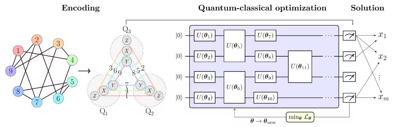 En Avvildung 1 us [1] weed dat Max-Cut-Problem als Beispell för de Veranschaulichung vum PCE-Aansatz jenomme. Dat Max-Cut-Problem met Knottepünkt weed en ene Pauli-Korrelationsraum kodeet, wobei dat Optimierungsproblem als Korrelationsmatrix dorjeställt weed, besonders als 2-Körper-Pauli-Matrix-Korrelationä üvver Qubits . Knottepünktfaave zeije dä Pauli-String aan, dä för jidde kodeet Knottepünkt jenomme weed.
Zom Beispell weed Knottepünkt 1, dä dä binääre Variabele entspreech, durch dä Erwartungswäät vun kodeet, während durch kodeet weed.
Dat entspreech ener Kompression vun dä Variable vum Problem en Qubits. Alljeemein ermöhliche -Körper-Korrelationä polynomielle Kompressione vun dä Ordnung . Dä jewählte Pauli-Satz ömfasst drei Deelmenge vun jejejenseidigg kommutierenden Pauli-Strings, woduurch all Korrelationä experimentell met blooß drei Messeinstellunge jeschätzt weede künne.
En Avvildung 1 us [1] weed dat Max-Cut-Problem als Beispell för de Veranschaulichung vum PCE-Aansatz jenomme. Dat Max-Cut-Problem met Knottepünkt weed en ene Pauli-Korrelationsraum kodeet, wobei dat Optimierungsproblem als Korrelationsmatrix dorjeställt weed, besonders als 2-Körper-Pauli-Matrix-Korrelationä üvver Qubits . Knottepünktfaave zeije dä Pauli-String aan, dä för jidde kodeet Knottepünkt jenomme weed.
Zom Beispell weed Knottepünkt 1, dä dä binääre Variabele entspreech, durch dä Erwartungswäät vun kodeet, während durch kodeet weed.
Dat entspreech ener Kompression vun dä Variable vum Problem en Qubits. Alljeemein ermöhliche -Körper-Korrelationä polynomielle Kompressione vun dä Ordnung . Dä jewählte Pauli-Satz ömfasst drei Deelmenge vun jejejenseidigg kommutierenden Pauli-Strings, woduurch all Korrelationä experimentell met blooß drei Messeinstellunge jeschätzt weede künne.
En Verlusfunktion vun Pauli-Erwartungswääte, di de ursprüngleche Max-Cut-Zielfunktion nohahmt, weed konstrueet. De Verlusfunktion weed dann met enem quante-klassische Optimierungsläuser wi däm Variational Quantum Eigensolver (VQE) optimeet.
Soobald de Optimierung avjeschlosse es, weed de Läusung en dä ursprüngleche Optimierungsraum retuurjekodeet, woduurch de optimale Max-Cut-Läusung errich weed.
Aanforderunge
Vür däm Aafang vun däm Tutorial stellt sescher, dat Ehr dat Folljende instaleet han:
- Qiskit SDK v1.0 oder hüüher, met Visualisierungs-Ungerstötzung
- Qiskit Runtime v0.22 oder hüüher (
pip install qiskit-ibm-runtime)
Enrichtung
# Added by doQumentation — required packages for this notebook
!pip install -q networkx numpy qiskit qiskit-ibm-runtime rustworkx scipy
from itertools import combinations

import numpy as np
import rustworkx as rx
from scipy.optimize import minimize

from qiskit.circuit.library import efficient_su2
from qiskit.transpiler.preset_passmanagers import generate_preset_pass_manager
from qiskit.quantum_info import SparsePauliOp
from qiskit_ibm_runtime import EstimatorV2 as Estimator
from qiskit_ibm_runtime import QiskitRuntimeService
from qiskit_ibm_runtime import Session
from rustworkx.visualization import mpl_draw

service = QiskitRuntimeService()
backend = service.least_busy(
    operational=True, simulator=False, min_num_qubits=127
)
def calc_cut_size(graph, partition0, partition1):
    """Calculate the cut size of the given partitions of the graph."""

    cut_size = 0
    for edge0, edge1 in graph.edge_list():
        if edge0 in partition0 and edge1 in partition1:
            cut_size += 1
        elif edge0 in partition1 and edge1 in partition0:
            cut_size += 1
    return cut_size
Schrett 1: Klassische Engaabe op e Quanteproblem avbelde
Max-Cut-Problem
Dat Max-Cut-Problem es e kombinatorisch Optimierungsproblem, dat op enem Graafe defineet es, wobei de Menge vun dä Knottepünkt un de Menge vun dä Kante es. Dat Ziel es et, de Knottepünkt en zweu Menge un ze partitioneere, esu dat de Aanzahl vun dä Kante zwesche dä zweu Menge maximeet weed. För en usföhleche Beschrievung vum Max-Cut-Problem luurt ens noh däm Tutorial "Quantum approximate optimization algorithm". Dodozou weed dat Max-Cut-Problem als Beispell em Tutorial "Advanced Techniques for QAOA" jenomme. En dänne Tutorials weed dä QAOA-Algorithmus för de Läusung vum Max-Cut-Problem enjjesatzt.
Graaf -> Hamiltonian
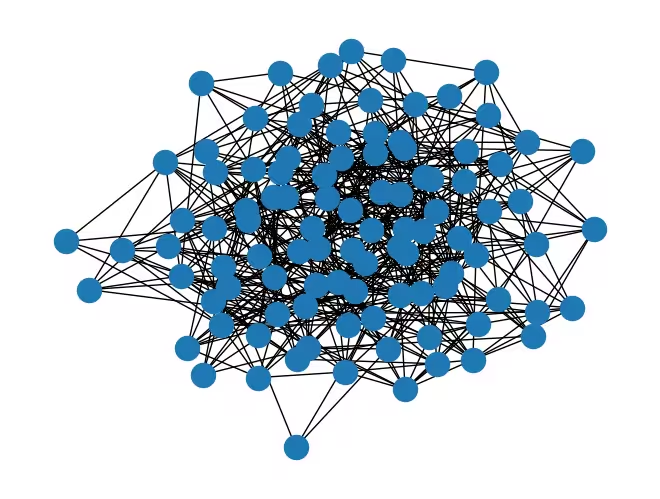
Dat Tutorial nötzt ene Zoofallsgraafe met 1000 Knottepünkt.
De Problemjrüüße es müjjelechwies schweer ze visualiseere, doröm es ungerwäärz ene Graaf met 100 Knottepünkt dorjeställt. (De direkte Dorstellung vun enem Graafe met 1.000 Knottepünkt dääd en zo dich maache, öm jet ze sinn!) Dä Graaf, met däm mer schaffe, es zehnmol jrüßer.
mpl_draw(rx.undirected_gnp_random_graph(100, 0.1, seed=42))
num_nodes = 1000  # Number of nodes in graph
graph = rx.undirected_gnp_random_graph(num_nodes, 0.1, seed=42)
import networkx as nx

nx_graph = nx.Graph()
nx_graph.add_nodes_from(range(num_nodes))
for edge in graph.edge_list():
    nx_graph.add_edge(edge[0], edge[1])
curr_cut_size, partition = nx.approximation.one_exchange(nx_graph, seed=1)
print(f"Initial cut size: {curr_cut_size}")
Initial cut size: 28075
Mer kodeere dä Graafe met 1000 Knottepünkt en 2-Körper-Pauli-Matrix-Korrelationä üvver 100 Qubits. Dä Graaf weed als Korrelationsmatrix dorjeställt, wobei jidde Knottepünkt durch ene Pauli-String kodeet weed. Dat Vüürzeiche vum Erwartungswäät vum Pauli-String jitt de Partition vum Knottepünkt aan. Zom Beispell weed Knottepünkt 0 durch ene Pauli-String kodeet, . Dat Vüürzeiche vum Erwartungswäät vun däm Pauli-String jitt de Partition vun Knottepünkt 0 aan. Mer defeneere e Pauli-Korrelations-Encoding (PCE) relativ zo als
wobei de Partition vun Knottepünkt es un dä Erwartungswäät vum Pauli-String es, dä Knottepünkt üvver ene Quantezustand kodeet. Jetz kodeere mer dä Graafe met PCE en ene Hamiltonian. Mer deele de Knottepünkt en drei Menge op: , un . Dann kodeere mer de Knottepünkt en jiddere Menge met dä Pauli-Strings , bzw. .
num_qubits = 100

list_size = num_nodes // 3
node_x = [i for i in range(list_size)]
node_y = [i for i in range(list_size, 2 * list_size)]
node_z = [i for i in range(2 * list_size, num_nodes)]

print("List 1:", node_x)
print("List 2:", node_y)
print("List 3:", node_z)
List 1: [0, 1, 2, 3, 4, 5, 6, 7, 8, 9, 10, 11, 12, 13, 14, 15, 16, 17, 18, 19, 20, 21, 22, 23, 24, 25, 26, 27, 28, 29, 30, 31, 32, 33, 34, 35, 36, 37, 38, 39, 40, 41, 42, 43, 44, 45, 46, 47, 48, 49, 50, 51, 52, 53, 54, 55, 56, 57, 58, 59, 60, 61, 62, 63, 64, 65, 66, 67, 68, 69, 70, 71, 72, 73, 74, 75, 76, 77, 78, 79, 80, 81, 82, 83, 84, 85, 86, 87, 88, 89, 90, 91, 92, 93, 94, 95, 96, 97, 98, 99, 100, 101, 102, 103, 104, 105, 106, 107, 108, 109, 110, 111, 112, 113, 114, 115, 116, 117, 118, 119, 120, 121, 122, 123, 124, 125, 126, 127, 128, 129, 130, 131, 132, 133, 134, 135, 136, 137, 138, 139, 140, 141, 142, 143, 144, 145, 146, 147, 148, 149, 150, 151, 152, 153, 154, 155, 156, 157, 158, 159, 160, 161, 162, 163, 164, 165, 166, 167, 168, 169, 170, 171, 172, 173, 174, 175, 176, 177, 178, 179, 180, 181, 182, 183, 184, 185, 186, 187, 188, 189, 190, 191, 192, 193, 194, 195, 196, 197, 198, 199, 200, 201, 202, 203, 204, 205, 206, 207, 208, 209, 210, 211, 212, 213, 214, 215, 216, 217, 218, 219, 220, 221, 222, 223, 224, 225, 226, 227, 228, 229, 230, 231, 232, 233, 234, 235, 236, 237, 238, 239, 240, 241, 242, 243, 244, 245, 246, 247, 248, 249, 250, 251, 252, 253, 254, 255, 256, 257, 258, 259, 260, 261, 262, 263, 264, 265, 266, 267, 268, 269, 270, 271, 272, 273, 274, 275, 276, 277, 278, 279, 280, 281, 282, 283, 284, 285, 286, 287, 288, 289, 290, 291, 292, 293, 294, 295, 296, 297, 298, 299, 300, 301, 302, 303, 304, 305, 306, 307, 308, 309, 310, 311, 312, 313, 314, 315, 316, 317, 318, 319, 320, 321, 322, 323, 324, 325, 326, 327, 328, 329, 330, 331, 332]
List 2: [333, 334, 335, 336, 337, 338, 339, 340, 341, 342, 343, 344, 345, 346, 347, 348, 349, 350, 351, 352, 353, 354, 355, 356, 357, 358, 359, 360, 361, 362, 363, 364, 365, 366, 367, 368, 369, 370, 371, 372, 373, 374, 375, 376, 377, 378, 379, 380, 381, 382, 383, 384, 385, 386, 387, 388, 389, 390, 391, 392, 393, 394, 395, 396, 397, 398, 399, 400, 401, 402, 403, 404, 405, 406, 407, 408, 409, 410, 411, 412, 413, 414, 415, 416, 417, 418, 419, 420, 421, 422, 423, 424, 425, 426, 427, 428, 429, 430, 431, 432, 433, 434, 435, 436, 437, 438, 439, 440, 441, 442, 443, 444, 445, 446, 447, 448, 449, 450, 451, 452, 453, 454, 455, 456, 457, 458, 459, 460, 461, 462, 463, 464, 465, 466, 467, 468, 469, 470, 471, 472, 473, 474, 475, 476, 477, 478, 479, 480, 481, 482, 483, 484, 485, 486, 487, 488, 489, 490, 491, 492, 493, 494, 495, 496, 497, 498, 499, 500, 501, 502, 503, 504, 505, 506, 507, 508, 509, 510, 511, 512, 513, 514, 515, 516, 517, 518, 519, 520, 521, 522, 523, 524, 525, 526, 527, 528, 529, 530, 531, 532, 533, 534, 535, 536, 537, 538, 539, 540, 541, 542, 543, 544, 545, 546, 547, 548, 549, 550, 551, 552, 553, 554, 555, 556, 557, 558, 559, 560, 561, 562, 563, 564, 565, 566, 567, 568, 569, 570, 571, 572, 573, 574, 575, 576, 577, 578, 579, 580, 581, 582, 583, 584, 585, 586, 587, 588, 589, 590, 591, 592, 593, 594, 595, 596, 597, 598, 599, 600, 601, 602, 603, 604, 605, 606, 607, 608, 609, 610, 611, 612, 613, 614, 615, 616, 617, 618, 619, 620, 621, 622, 623, 624, 625, 626, 627, 628, 629, 630, 631, 632, 633, 634, 635, 636, 637, 638, 639, 640, 641, 642, 643, 644, 645, 646, 647, 648, 649, 650, 651, 652, 653, 654, 655, 656, 657, 658, 659, 660, 661, 662, 663, 664, 665]
List 3: [666, 667, 668, 669, 670, 671, 672, 673, 674, 675, 676, 677, 678, 679, 680, 681, 682, 683, 684, 685, 686, 687, 688, 689, 690, 691, 692, 693, 694, 695, 696, 697, 698, 699, 700, 701, 702, 703, 704, 705, 706, 707, 708, 709, 710, 711, 712, 713, 714, 715, 716, 717, 718, 719, 720, 721, 722, 723, 724, 725, 726, 727, 728, 729, 730, 731, 732, 733, 734, 735, 736, 737, 738, 739, 740, 741, 742, 743, 744, 745, 746, 747, 748, 749, 750, 751, 752, 753, 754, 755, 756, 757, 758, 759, 760, 761, 762, 763, 764, 765, 766, 767, 768, 769, 770, 771, 772, 773, 774, 775, 776, 777, 778, 779, 780, 781, 782, 783, 784, 785, 786, 787, 788, 789, 790, 791, 792, 793, 794, 795, 796, 797, 798, 799, 800, 801, 802, 803, 804, 805, 806, 807, 808, 809, 810, 811, 812, 813, 814, 815, 816, 817, 818, 819, 820, 821, 822, 823, 824, 825, 826, 827, 828, 829, 830, 831, 832, 833, 834, 835, 836, 837, 838, 839, 840, 841, 842, 843, 844, 845, 846, 847, 848, 849, 850, 851, 852, 853, 854, 855, 856, 857, 858, 859, 860, 861, 862, 863, 864, 865, 866, 867, 868, 869, 870, 871, 872, 873, 874, 875, 876, 877, 878, 879, 880, 881, 882, 883, 884, 885, 886, 887, 888, 889, 890, 891, 892, 893, 894, 895, 896, 897, 898, 899, 900, 901, 902, 903, 904, 905, 906, 907, 908, 909, 910, 911, 912, 913, 914, 915, 916, 917, 918, 919, 920, 921, 922, 923, 924, 925, 926, 927, 928, 929, 930, 931, 932, 933, 934, 935, 936, 937, 938, 939, 940, 941, 942, 943, 944, 945, 946, 947, 948, 949, 950, 951, 952, 953, 954, 955, 956, 957, 958, 959, 960, 961, 962, 963, 964, 965, 966, 967, 968, 969, 970, 971, 972, 973, 974, 975, 976, 977, 978, 979, 980, 981, 982, 983, 984, 985, 986, 987, 988, 989, 990, 991, 992, 993, 994, 995, 996, 997, 998, 999]
def build_pauli_correlation_encoding(pauli, node_list, n, k=2):
    pauli_correlation_encoding = []
    for idx, c in enumerate(combinations(range(n), k)):
        if idx >= len(node_list):
            break
        paulis = ["I"] * n
        paulis[c[0]], paulis[c[1]] = pauli, pauli
        pauli_correlation_encoding.append(("".join(paulis)[::-1], 1))

    hamiltonian = []
    for pauli, weight in pauli_correlation_encoding:
        hamiltonian.append(SparsePauliOp.from_list([(pauli, weight)]))

    return hamiltonian

pauli_correlation_encoding_x = build_pauli_correlation_encoding(
    "X", node_x, num_qubits
)
pauli_correlation_encoding_y = build_pauli_correlation_encoding(
    "Y", node_y, num_qubits
)
pauli_correlation_encoding_z = build_pauli_correlation_encoding(
    "Z", node_z, num_qubits
)
Schrett 2: Problem för de Usföhrung op Quante-Hardware optimiere
Quanteschaltkreis
Hee weed dä Zustand met parametriseet, un mer optimiere dänne Parameter met enem variationelle Aansatz.
Dat Tutorial nötzt dä efficient_su2 Aansatz för onge variationelle Algorithmus wäje singe Usdrucksfähigkeit un einfache Implementierung.
Mer nemme och de relaxete Verlusfunktion, di später em Tutorial enjeföhrt weed.
Als Erjebnis künne mer jrußskalige Probleme met weinijer Qubits un jeringjere Schaltkreistieffe aajohn.
# Build the quantum circuit
qc = efficient_su2(num_qubits, ["ry", "rz"], reps=2)
# Optimize the circuit

pm = generate_preset_pass_manager(optimization_level=3, backend=backend)
qc = pm.run(qc)
Verlusfunktion
För de Verlusfunktion nemme mer en Relaxation vun dä Max-Cut-Zielfunktion wi en [1] beschrevve, di als defineet es. Hee bezeichnet dat Jewich vun dä Kante un de Partition vun Knottepünkt . De Verlusfunktion es jejovve durch:
wobei de Max-Cut-Zielfunktion durch jlatte hyperbolische Tangente vun dä Erwartungswääte vun dä Pauli-Strings ersatz weed, di de Knottepünkt kodeere. Dä Regularisierungsterm un dä Skalierungsfaktor , proportional zo dä Aanzahl vun dä Qubits, weede enjeföhrt, öm de Leistung vum Läuser ze verbessere.
Dä Regularisierungsterm es defineet als:
es defineet als
wobei , un de Aanzahl vun dä Knottepünkt em Graafe es.
def loss_func_estimator(x, ansatz, hamiltonian, estimator, graph):
    """
    Calculates the specified loss function for the given ansatz, Hamiltonian, and graph.

    The expectation values of each Pauli string in the Hamiltonian are first obtained
    by running the ansatz on the quantum backend. These expectation values are then
    passed through the nonlinear function tanh(alpha * prod_i). The loss function is
    subsequently computed from these transformed values.
    """
    job = estimator.run(
        [
            (ansatz, hamiltonian[0], x),
            (ansatz, hamiltonian[1], x),
            (ansatz, hamiltonian[2], x),
        ]
    )
    result = job.result()

    # calculate the loss function
    node_exp_map = {}
    idx = 0
    for r in result:
        for ev in r.data.evs:
            node_exp_map[idx] = ev
            idx += 1

    loss = 0
    alpha = num_qubits
    for edge0, edge1 in graph.edge_list():
        loss += np.tanh(alpha * node_exp_map[edge0]) * np.tanh(
            alpha * node_exp_map[edge1]
        )

    regulation_term = 0
    for i in range(len(graph.nodes())):
        regulation_term += np.tanh(alpha * node_exp_map[i]) ** 2
    regulation_term = regulation_term / len(graph.nodes())
    regulation_term = regulation_term**2
    beta = 1 / 2
    v = len(graph.edges()) / 2 + (len(graph.nodes()) - 1) / 4
    regulation_term = beta * v * regulation_term

    loss = loss + regulation_term

    global experiment_result
    print(f"Iter {len(experiment_result)}: {loss}")
    experiment_result.append({"loss": loss, "exp_map": node_exp_map})
    return loss
Schrett 3: Usföhrung met Qiskit Primitives
En däm Tutorial setze mer max_iter=50 för de Optimierungsschleif för Demonstrationszwecke. Wann mer de Aanzahl vun dä Iterationä erhüühe, künne mer bessere Erjbnisse verwade.
pce = []
pce.append(
    [op.apply_layout(qc.layout) for op in pauli_correlation_encoding_x]
)
pce.append(
    [op.apply_layout(qc.layout) for op in pauli_correlation_encoding_y]
)
pce.append(
    [op.apply_layout(qc.layout) for op in pauli_correlation_encoding_z]
)
# Run the optimization using Session

with Session(backend=backend) as session:
    estimator = Estimator(mode=session)

    experiment_result = []

    def loss_func(x):
        return loss_func_estimator(
            x, qc, [pce[0], pce[1], pce[2]], estimator, graph
        )

    np.random.seed(42)
    initial_params = np.random.rand(qc.num_parameters)
    result = minimize(
        loss_func, initial_params, method="COBYLA", options={"maxiter": 50}
    )
print(result)
Iter 0: 16659.649201600296
Iter 1: 12104.242957555361
Iter 2: 6541.137221994661
Iter 3: 6650.6188244671985
Iter 4: 7033.193518185085
Iter 5: 6743.687931793412
Iter 6: 6223.574718684094
Iter 7: 6457.3302709535965
Iter 8: 6581.316449107595
Iter 9: 6365.761052029896
Iter 10: 6415.872673527322
Iter 11: 6421.996561600348
Iter 12: 6636.372822791712
Iter 13: 6965.174320702346
Iter 14: 6774.236562696287
Iter 15: 6393.837617108355
Iter 16: 6234.311401676519
Iter 17: 6518.192237615901
Iter 18: 6559.933925068997
Iter 19: 6646.157979243488
Iter 20: 6573.726111605048
Iter 21: 6190.642092901959
Iter 22: 6653.06500163594
Iter 23: 6545.713700369988
Iter 24: 6399.996441760465
Iter 25: 6115.959687941808
Iter 26: 6665.915093554849
Iter 27: 6832.882201259893
Iter 28: 6541.392749578919
Iter 29: 6813.3456910443165
Iter 30: 6460.800944368402
Iter 31: 6359.635437029245
Iter 32: 6040.891641882451
Iter 33: 6573.930674936448
Iter 34: 6668.031753293785
Iter 35: 6450.002712889748
Iter 36: 6519.8298811058075
Iter 37: 6467.134502398199
Iter 38: 6655.284651397334
Iter 39: 6371.168353987336
Iter 40: 6480.337259347923
Iter 41: 6339.256786764425
Iter 42: 6588.635046825541
Iter 43: 6617.677964971322
Iter 44: 6469.0441600679205
Iter 45: 6567.874244906106
Iter 46: 6217.899975264532
Iter 47: 6783.481394627947
Iter 48: 6813.371853626112
Iter 49: 6506.5871531488765
 message: Maximum number of function evaluations has been exceeded.
 success: False
  status: 2
     fun: 6040.891641882451
       x: [ 1.375e+00  1.951e+00 ...  1.923e-01  4.087e-02]
    nfev: 50
   maxcv: 0.0
Schrett 4: Nohbeärbeitung un Retuurjaab vum Erjebnis em jewönschte klassische Format
De Partitionä vun dä Knottepünkt weede durch Uswätung vum Vüürzeiche vun dä Erwartungswääte vun dä Pauli-Strings bestimmt, di de Knottepünkt kodeere.
# Calculate the partitions based on the final expectation values
# If the expectation value is positive, the node belongs to partition 0 (par0)
# Otherwise, the node belongs to partition 1 (par1)

par0, par1 = set(), set()

for i in experiment_result[-1]["exp_map"]:
    if experiment_result[-1]["exp_map"][i] >= 0:
        par0.add(i)
    else:
        par1.add(i)
print(par0, par1)
{0, 1, 4, 8, 9, 10, 12, 13, 14, 15, 16, 18, 25, 27, 31, 32, 34, 36, 38, 39, 40, 41, 44, 46, 47, 48, 49, 50, 51, 52, 57, 60, 61, 62, 63, 64, 65, 66, 68, 71, 79, 81, 82, 86, 88, 91, 92, 93, 94, 95, 96, 99, 100, 105, 106, 107, 112, 114, 115, 121, 123, 129, 133, 134, 145, 147, 161, 165, 166, 168, 171, 173, 184, 185, 187, 188, 192, 193, 194, 196, 197, 198, 202, 205, 206, 207, 208, 209, 210, 211, 215, 217, 218, 219, 220, 221, 225, 226, 227, 228, 229, 230, 231, 232, 233, 234, 235, 236, 238, 241, 242, 243, 244, 246, 247, 248, 249, 251, 252, 253, 255, 256, 257, 258, 259, 261, 262, 264, 265, 266, 268, 269, 270, 272, 273, 275, 276, 277, 278, 279, 281, 283, 284, 285, 286, 288, 292, 293, 294, 299, 300, 303, 305, 306, 307, 308, 310, 312, 313, 314, 316, 317, 319, 321, 326, 327, 328, 333, 336, 338, 340, 341, 342, 344, 345, 346, 349, 351, 352, 353, 356, 357, 360, 361, 362, 363, 364, 366, 368, 370, 374, 378, 379, 380, 381, 382, 383, 384, 386, 387, 388, 389, 390, 391, 393, 394, 395, 396, 397, 398, 404, 405, 406, 409, 411, 413, 415, 416, 418, 421, 425, 426, 427, 428, 429, 433, 434, 435, 437, 444, 450, 456, 457, 458, 459, 462, 463, 465, 467, 469, 470, 472, 476, 479, 484, 487, 489, 492, 493, 497, 498, 499, 502, 506, 508, 513, 516, 517, 518, 519, 521, 523, 526, 527, 528, 531, 532, 533, 535, 536, 537, 539, 540, 541, 542, 543, 544, 545, 547, 549, 550, 552, 557, 562, 563, 564, 565, 567, 568, 569, 570, 571, 572, 573, 576, 578, 579, 580, 583, 585, 587, 588, 589, 591, 595, 596, 597, 600, 602, 603, 604, 605, 606, 607, 608, 609, 610, 612, 618, 619, 623, 624, 625, 626, 627, 628, 630, 632, 636, 637, 640, 644, 646, 649, 652, 656, 657, 658, 659, 661, 662, 663, 664, 667, 669, 670, 671, 672, 674, 675, 676, 677, 678, 679, 680, 681, 682, 683, 684, 685, 686, 687, 688, 689, 690, 692, 693, 694, 695, 696, 698, 700, 701, 703, 706, 707, 708, 709, 712, 713, 714, 716, 717, 718, 719, 721, 722, 723, 724, 725, 726, 728, 730, 731, 733, 734, 735, 737, 739, 740, 741, 743, 744, 746, 748, 750, 751, 752, 753, 754, 758, 760, 761, 762, 763, 764, 765, 766, 774, 778, 780, 782, 787, 795, 800, 802, 803, 808, 809, 812, 818, 822, 825, 827, 834, 836, 840, 843, 845, 847, 850, 853, 854, 857, 858, 863, 864, 865, 866, 867, 868, 869, 870, 872, 873, 874, 875, 876, 878, 880, 881, 882, 883, 884, 885, 887, 888, 889, 890, 891, 893, 894, 895, 896, 898, 901, 902, 903, 904, 905, 907, 908, 910, 911, 912, 913, 914, 915, 916, 917, 918, 920, 921, 923, 925, 926, 928, 929, 930, 932, 934, 935, 936, 938, 939, 941, 943, 945, 946, 947, 948, 949, 953, 955, 956, 957, 958, 959, 961, 966, 975, 978, 980, 983, 988, 990, 996, 999} {2, 3, 5, 6, 7, 11, 17, 19, 20, 21, 22, 23, 24, 26, 28, 29, 30, 33, 35, 37, 42, 43, 45, 53, 54, 55, 56, 58, 59, 67, 69, 70, 72, 73, 74, 75, 76, 77, 78, 80, 83, 84, 85, 87, 89, 90, 97, 98, 101, 102, 103, 104, 108, 109, 110, 111, 113, 116, 117, 118, 119, 120, 122, 124, 125, 126, 127, 128, 130, 131, 132, 135, 136, 137, 138, 139, 140, 141, 142, 143, 144, 146, 148, 149, 150, 151, 152, 153, 154, 155, 156, 157, 158, 159, 160, 162, 163, 164, 167, 169, 170, 172, 174, 175, 176, 177, 178, 179, 180, 181, 182, 183, 186, 189, 190, 191, 195, 199, 200, 201, 203, 204, 212, 213, 214, 216, 222, 223, 224, 237, 239, 240, 245, 250, 254, 260, 263, 267, 271, 274, 280, 282, 287, 289, 290, 291, 295, 296, 297, 298, 301, 302, 304, 309, 311, 315, 318, 320, 322, 323, 324, 325, 329, 330, 331, 332, 334, 335, 337, 339, 343, 347, 348, 350, 354, 355, 358, 359, 365, 367, 369, 371, 372, 373, 375, 376, 377, 385, 392, 399, 400, 401, 402, 403, 407, 408, 410, 412, 414, 417, 419, 420, 422, 423, 424, 430, 431, 432, 436, 438, 439, 440, 441, 442, 443, 445, 446, 447, 448, 449, 451, 452, 453, 454, 455, 460, 461, 464, 466, 468, 471, 473, 474, 475, 477, 478, 480, 481, 482, 483, 485, 486, 488, 490, 491, 494, 495, 496, 500, 501, 503, 504, 505, 507, 509, 510, 511, 512, 514, 515, 520, 522, 524, 525, 529, 530, 534, 538, 546, 548, 551, 553, 554, 555, 556, 558, 559, 560, 561, 566, 574, 575, 577, 581, 582, 584, 586, 590, 592, 593, 594, 598, 599, 601, 611, 613, 614, 615, 616, 617, 620, 621, 622, 629, 631, 633, 634, 635, 638, 639, 641, 642, 643, 645, 647, 648, 650, 651, 653, 654, 655, 660, 665, 666, 668, 673, 691, 697, 699, 702, 704, 705, 710, 711, 715, 720, 727, 729, 732, 736, 738, 742, 745, 747, 749, 755, 756, 757, 759, 767, 768, 769, 770, 771, 772, 773, 775, 776, 777, 779, 781, 783, 784, 785, 786, 788, 789, 790, 791, 792, 793, 794, 796, 797, 798, 799, 801, 804, 805, 806, 807, 810, 811, 813, 814, 815, 816, 817, 819, 820, 821, 823, 824, 826, 828, 829, 830, 831, 832, 833, 835, 837, 838, 839, 841, 842, 844, 846, 848, 849, 851, 852, 855, 856, 859, 860, 861, 862, 871, 877, 879, 886, 892, 897, 899, 900, 906, 909, 919, 922, 924, 927, 931, 933, 937, 940, 942, 944, 950, 951, 952, 954, 960, 962, 963, 964, 965, 967, 968, 969, 970, 971, 972, 973, 974, 976, 977, 979, 981, 982, 984, 985, 986, 987, 989, 991, 992, 993, 994, 995, 997, 998}
Mer künne de Cut-Jrüüße vum Max-Cut-Problem met dä Partitionä vun dä Knottepünkt berechne.
cut_size = calc_cut_size(graph, par0, par1)
print(f"Cut size: {cut_size}")
Cut size: 24682
Soobald dat Training avjeschlosse es, fohre mer en Runde Single-Bit-Swap-Such durch, öm de Läusung als klassische Nohbeärbeidungsschrett ze verbessere. Bei däm Prozess verdausche mer de Partitionä vun zweu Knottepünkt un bewäde de Cut-Jrüüße. Wann de Cut-Jrüüße verbessert weed, behalde mer dä Dausch. Mer widderhohle dänne Prozess för all müjjeleche Knottepünktpore, di durch en Kant verbunge sin.
best_bits = []
cur_bits = []

for i in experiment_result[-1]["exp_map"]:
    if experiment_result[-1]["exp_map"][i] >= 0:
        cur_bits.append(1)
    else:
        cur_bits.append(0)
print(cur_bits)
[1, 1, 0, 0, 1, 0, 0, 0, 1, 1, 1, 0, 1, 1, 1, 1, 1, 0, 1, 0, 0, 0, 0, 0, 0, 1, 0, 1, 0, 0, 0, 1, 1, 0, 1, 0, 1, 0, 1, 1, 1, 1, 0, 0, 1, 0, 1, 1, 1, 1, 1, 1, 1, 0, 0, 0, 0, 1, 0, 0, 1, 1, 1, 1, 1, 1, 1, 0, 1, 0, 0, 1, 0, 0, 0, 0, 0, 0, 0, 1, 0, 1, 1, 0, 0, 0, 1, 0, 1, 0, 0, 1, 1, 1, 1, 1, 1, 0, 0, 1, 1, 0, 0, 0, 0, 1, 1, 1, 0, 0, 0, 0, 1, 0, 1, 1, 0, 0, 0, 0, 0, 1, 0, 1, 0, 0, 0, 0, 0, 1, 0, 0, 0, 1, 1, 0, 0, 0, 0, 0, 0, 0, 0, 0, 0, 1, 0, 1, 0, 0, 0, 0, 0, 0, 0, 0, 0, 0, 0, 0, 0, 1, 0, 0, 0, 1, 1, 0, 1, 0, 0, 1, 0, 1, 0, 0, 0, 0, 0, 0, 0, 0, 0, 0, 1, 1, 0, 1, 1, 0, 0, 0, 1, 1, 1, 0, 1, 1, 1, 0, 0, 0, 1, 0, 0, 1, 1, 1, 1, 1, 1, 1, 0, 0, 0, 1, 0, 1, 1, 1, 1, 1, 0, 0, 0, 1, 1, 1, 1, 1, 1, 1, 1, 1, 1, 1, 1, 0, 1, 0, 0, 1, 1, 1, 1, 0, 1, 1, 1, 1, 0, 1, 1, 1, 0, 1, 1, 1, 1, 1, 0, 1, 1, 0, 1, 1, 1, 0, 1, 1, 1, 0, 1, 1, 0, 1, 1, 1, 1, 1, 0, 1, 0, 1, 1, 1, 1, 0, 1, 0, 0, 0, 1, 1, 1, 0, 0, 0, 0, 1, 1, 0, 0, 1, 0, 1, 1, 1, 1, 0, 1, 0, 1, 1, 1, 0, 1, 1, 0, 1, 0, 1, 0, 0, 0, 0, 1, 1, 1, 0, 0, 0, 0, 1, 0, 0, 1, 0, 1, 0, 1, 1, 1, 0, 1, 1, 1, 0, 0, 1, 0, 1, 1, 1, 0, 0, 1, 1, 0, 0, 1, 1, 1, 1, 1, 0, 1, 0, 1, 0, 1, 0, 0, 0, 1, 0, 0, 0, 1, 1, 1, 1, 1, 1, 1, 0, 1, 1, 1, 1, 1, 1, 0, 1, 1, 1, 1, 1, 1, 0, 0, 0, 0, 0, 1, 1, 1, 0, 0, 1, 0, 1, 0, 1, 0, 1, 1, 0, 1, 0, 0, 1, 0, 0, 0, 1, 1, 1, 1, 1, 0, 0, 0, 1, 1, 1, 0, 1, 0, 0, 0, 0, 0, 0, 1, 0, 0, 0, 0, 0, 1, 0, 0, 0, 0, 0, 1, 1, 1, 1, 0, 0, 1, 1, 0, 1, 0, 1, 0, 1, 1, 0, 1, 0, 0, 0, 1, 0, 0, 1, 0, 0, 0, 0, 1, 0, 0, 1, 0, 1, 0, 0, 1, 1, 0, 0, 0, 1, 1, 1, 0, 0, 1, 0, 0, 0, 1, 0, 1, 0, 0, 0, 0, 1, 0, 0, 1, 1, 1, 1, 0, 1, 0, 1, 0, 0, 1, 1, 1, 0, 0, 1, 1, 1, 0, 1, 1, 1, 0, 1, 1, 1, 1, 1, 1, 1, 0, 1, 0, 1, 1, 0, 1, 0, 0, 0, 0, 1, 0, 0, 0, 0, 1, 1, 1, 1, 0, 1, 1, 1, 1, 1, 1, 1, 0, 0, 1, 0, 1, 1, 1, 0, 0, 1, 0, 1, 0, 1, 1, 1, 0, 1, 0, 0, 0, 1, 1, 1, 0, 0, 1, 0, 1, 1, 1, 1, 1, 1, 1, 1, 1, 0, 1, 0, 0, 0, 0, 0, 1, 1, 0, 0, 0, 1, 1, 1, 1, 1, 1, 0, 1, 0, 1, 0, 0, 0, 1, 1, 0, 0, 1, 0, 0, 0, 1, 0, 1, 0, 0, 1, 0, 0, 1, 0, 0, 0, 1, 1, 1, 1, 0, 1, 1, 1, 1, 0, 0, 1, 0, 1, 1, 1, 1, 0, 1, 1, 1, 1, 1, 1, 1, 1, 1, 1, 1, 1, 1, 1, 1, 1, 1, 0, 1, 1, 1, 1, 1, 0, 1, 0, 1, 1, 0, 1, 0, 0, 1, 1, 1, 1, 0, 0, 1, 1, 1, 0, 1, 1, 1, 1, 0, 1, 1, 1, 1, 1, 1, 0, 1, 0, 1, 1, 0, 1, 1, 1, 0, 1, 0, 1, 1, 1, 0, 1, 1, 0, 1, 0, 1, 0, 1, 1, 1, 1, 1, 0, 0, 0, 1, 0, 1, 1, 1, 1, 1, 1, 1, 0, 0, 0, 0, 0, 0, 0, 1, 0, 0, 0, 1, 0, 1, 0, 1, 0, 0, 0, 0, 1, 0, 0, 0, 0, 0, 0, 0, 1, 0, 0, 0, 0, 1, 0, 1, 1, 0, 0, 0, 0, 1, 1, 0, 0, 1, 0, 0, 0, 0, 0, 1, 0, 0, 0, 1, 0, 0, 1, 0, 1, 0, 0, 0, 0, 0, 0, 1, 0, 1, 0, 0, 0, 1, 0, 0, 1, 0, 1, 0, 1, 0, 0, 1, 0, 0, 1, 1, 0, 0, 1, 1, 0, 0, 0, 0, 1, 1, 1, 1, 1, 1, 1, 1, 0, 1, 1, 1, 1, 1, 0, 1, 0, 1, 1, 1, 1, 1, 1, 0, 1, 1, 1, 1, 1, 0, 1, 1, 1, 1, 0, 1, 0, 0, 1, 1, 1, 1, 1, 0, 1, 1, 0, 1, 1, 1, 1, 1, 1, 1, 1, 1, 0, 1, 1, 0, 1, 0, 1, 1, 0, 1, 1, 1, 0, 1, 0, 1, 1, 1, 0, 1, 1, 0, 1, 0, 1, 0, 1, 1, 1, 1, 1, 0, 0, 0, 1, 0, 1, 1, 1, 1, 1, 0, 1, 0, 0, 0, 0, 1, 0, 0, 0, 0, 0, 0, 0, 0, 1, 0, 0, 1, 0, 1, 0, 0, 1, 0, 0, 0, 0, 1, 0, 1, 0, 0, 0, 0, 0, 1, 0, 0, 1]
# Swap the partitions and calculate the cut size
best_cut = 0
for edge0, edge1 in graph.edge_list():
    swapped_bits = cur_bits.copy()
    swapped_bits[edge0], swapped_bits[edge1] = (
        swapped_bits[edge1],
        swapped_bits[edge0],
    )

    cur_partition = [set(), set()]
    for i, bit in enumerate(swapped_bits):
        if bit > 0:
            cur_partition[0].add(i)
        else:
            cur_partition[1].add(i)
    cut_size = calc_cut_size(graph, cur_partition[0], cur_partition[1])
    if best_cut < cut_size:
        best_cut = cut_size
        best_bits = swapped_bits

print(best_cut, best_bits)
24733 [1, 1, 0, 0, 1, 0, 0, 0, 1, 1, 1, 0, 1, 1, 1, 1, 1, 0, 1, 0, 0, 0, 0, 0, 0, 1, 0, 1, 0, 0, 0, 1, 1, 0, 1, 0, 1, 0, 1, 1, 1, 1, 0, 0, 1, 0, 1, 1, 1, 1, 1, 1, 1, 0, 0, 0, 0, 1, 0, 0, 1, 1, 1, 1, 1, 1, 1, 0, 1, 0, 0, 1, 0, 0, 0, 0, 0, 0, 0, 1, 0, 1, 1, 0, 0, 0, 1, 0, 1, 0, 0, 1, 1, 1, 1, 1, 1, 0, 0, 1, 1, 0, 0, 0, 0, 1, 1, 1, 0, 0, 0, 0, 1, 0, 1, 1, 0, 0, 0, 0, 0, 1, 0, 1, 0, 0, 0, 0, 0, 1, 0, 0, 0, 1, 1, 0, 0, 0, 0, 0, 0, 0, 0, 0, 0, 1, 0, 1, 0, 0, 0, 0, 0, 0, 0, 0, 0, 0, 0, 0, 0, 1, 0, 0, 0, 1, 1, 0, 1, 0, 0, 1, 0, 1, 0, 0, 0, 0, 0, 0, 0, 0, 0, 0, 1, 1, 0, 1, 1, 0, 0, 0, 1, 1, 1, 0, 1, 1, 1, 0, 0, 0, 1, 0, 0, 1, 1, 1, 1, 1, 1, 1, 0, 0, 0, 1, 0, 1, 1, 1, 1, 1, 0, 0, 0, 1, 1, 1, 1, 1, 1, 1, 1, 1, 1, 1, 1, 0, 1, 0, 0, 1, 1, 1, 1, 0, 0, 1, 1, 1, 0, 1, 1, 1, 0, 1, 1, 1, 1, 1, 0, 1, 1, 0, 1, 1, 1, 0, 1, 1, 1, 0, 1, 1, 0, 1, 1, 1, 1, 1, 0, 1, 0, 1, 1, 1, 1, 0, 1, 0, 0, 0, 1, 1, 1, 0, 0, 0, 0, 1, 1, 0, 0, 1, 0, 1, 1, 1, 1, 0, 1, 0, 1, 1, 1, 0, 1, 1, 0, 1, 0, 1, 0, 0, 0, 0, 1, 1, 1, 0, 0, 0, 0, 1, 0, 0, 1, 0, 1, 0, 1, 1, 1, 0, 1, 1, 1, 0, 0, 1, 0, 1, 1, 1, 0, 0, 1, 1, 0, 0, 1, 1, 1, 1, 1, 0, 1, 0, 1, 0, 1, 0, 0, 0, 1, 0, 0, 0, 1, 1, 1, 1, 1, 1, 1, 0, 1, 1, 1, 1, 1, 1, 0, 1, 1, 1, 1, 1, 1, 0, 0, 0, 0, 0, 1, 1, 1, 0, 0, 1, 0, 1, 0, 1, 0, 1, 1, 0, 1, 0, 0, 1, 0, 0, 0, 1, 1, 1, 1, 1, 0, 0, 0, 1, 1, 1, 0, 1, 0, 0, 0, 0, 0, 0, 1, 0, 0, 0, 0, 0, 1, 0, 0, 0, 0, 0, 1, 1, 1, 1, 0, 0, 1, 1, 0, 1, 0, 1, 0, 1, 1, 0, 1, 0, 0, 0, 1, 0, 0, 1, 0, 0, 0, 0, 1, 0, 0, 1, 0, 1, 0, 0, 1, 1, 0, 0, 0, 1, 1, 1, 0, 0, 1, 0, 0, 0, 1, 0, 1, 0, 0, 0, 0, 1, 0, 0, 1, 1, 1, 1, 0, 1, 0, 1, 0, 0, 1, 1, 1, 0, 0, 1, 1, 1, 0, 1, 1, 1, 0, 1, 1, 1, 1, 1, 1, 1, 0, 1, 0, 1, 1, 0, 1, 0, 0, 0, 0, 1, 0, 0, 0, 0, 1, 1, 1, 1, 0, 1, 1, 1, 1, 1, 1, 1, 0, 0, 1, 0, 1, 1, 1, 0, 0, 1, 0, 1, 0, 1, 1, 1, 0, 1, 0, 0, 0, 1, 1, 1, 0, 0, 1, 0, 1, 1, 1, 1, 1, 1, 1, 1, 1, 0, 1, 0, 0, 0, 0, 0, 1, 1, 0, 0, 0, 1, 1, 1, 1, 1, 1, 0, 1, 0, 1, 0, 1, 0, 1, 1, 0, 0, 1, 0, 0, 0, 1, 0, 1, 0, 0, 1, 0, 0, 1, 0, 0, 0, 1, 1, 1, 1, 0, 1, 1, 1, 1, 0, 0, 1, 0, 1, 1, 1, 1, 0, 1, 1, 1, 1, 1, 1, 1, 1, 1, 1, 1, 1, 1, 1, 1, 1, 1, 0, 1, 1, 1, 1, 1, 0, 1, 0, 1, 1, 0, 1, 0, 0, 1, 1, 1, 1, 0, 0, 1, 1, 1, 0, 1, 1, 1, 1, 0, 1, 1, 1, 1, 1, 1, 0, 1, 0, 1, 1, 0, 1, 1, 1, 0, 1, 0, 1, 1, 1, 0, 1, 1, 0, 1, 0, 1, 0, 1, 1, 1, 1, 1, 0, 0, 0, 1, 0, 1, 1, 1, 1, 1, 1, 1, 0, 0, 0, 0, 0, 0, 0, 1, 0, 0, 0, 1, 0, 1, 0, 1, 0, 0, 0, 0, 1, 0, 0, 0, 0, 0, 0, 0, 1, 0, 0, 0, 0, 1, 0, 1, 1, 0, 0, 0, 0, 1, 1, 0, 0, 1, 0, 0, 0, 0, 0, 1, 0, 0, 0, 1, 0, 0, 1, 0, 1, 0, 0, 0, 0, 0, 0, 1, 0, 1, 0, 0, 0, 1, 0, 0, 1, 0, 1, 0, 1, 0, 0, 1, 0, 0, 1, 1, 0, 0, 1, 1, 0, 0, 0, 0, 1, 1, 1, 1, 1, 1, 1, 1, 0, 1, 1, 1, 1, 1, 0, 1, 0, 1, 1, 1, 1, 1, 1, 0, 1, 1, 1, 1, 1, 0, 1, 1, 1, 1, 0, 1, 0, 0, 1, 1, 1, 1, 1, 0, 1, 1, 0, 1, 1, 1, 1, 1, 1, 1, 1, 1, 0, 1, 1, 0, 1, 0, 1, 1, 0, 1, 1, 1, 0, 1, 0, 1, 1, 1, 0, 1, 1, 0, 1, 0, 1, 0, 1, 1, 1, 1, 1, 0, 0, 0, 1, 0, 1, 1, 1, 1, 1, 0, 1, 0, 0, 0, 0, 1, 0, 0, 0, 0, 0, 0, 0, 0, 1, 0, 0, 1, 0, 1, 0, 0, 1, 0, 0, 0, 0, 1, 0, 1, 0, 0, 0, 0, 0, 1, 0, 0, 1]
Referenze
[1] Sciorilli, M., Borges, L., Patti, T. L., García-Martín, D., Camilo, G., Anandkumar, A., & Aolita, L. (2024). Towards large-scale quantum optimization solvers with few qubits. arXiv preprint arXiv:2401.09421.
Tutorial-Ömfraach
Bitte nemmt aan dä kooze Ömfraach del, öm Feedback zo däm Tutorial ze jevve. Ding Erkenntnisse hellefe os, onge Inhaltsaanjebode un Nötzererfahrung ze verbessere.